Short Questions:
Mean:
Mean is the sum of all the values of data set divided by the total number of values in the data set. It is the single value which is calculated to represent the whole set of data. The symbol $\bar{x}$ (read as “x bar”) represent the sample mean. The bar above the letter x represents the mean of a set of values.
Arithmetic Mean $= \bar{x} = \frac{\text{sum of values}}{\text{Total number of values}}$
Median:
The median is the middle value in a dataset that are arranged in ascending or descending order of magnitude. Median divides the data set into two equal parts. One part of the dataset have the values less than the middle value and the other part of the dataset have values greater than the middle item. It is denoted by $\tilde{x}$ (read as “x tilde” or “x snake”). It is necessary to arrange the values of dataset in ascending or descending order.
Mode:
The mode is the value in a dataset that appears maximum number of times. A dataset may have one mode (unimodal), more than one mode (bimodal or multimodal) or no mode at all (amodal) i.e., all values occur in same number of times. It may be denoted by “$\hat{x}$” (read as x-hat or x-cap).
Mode = the most frequent or repeated value occurring in a given dataset.
Formulae of median:
For dataset with odd number of value:
$$\text{Median }(\tilde{x}) = \left(\frac{n+1}{2}\right)^{\text{th}}$$
For dataset with even number of value:
$$\text{Median }(\tilde{x})=\frac{\left(\frac{n}{2}\text{th value}\right)+\left(\left(\frac{n}{2}+1\right)\text{th value}\right)}{2}$$
Formulae of mode:
$$\text{Mode }(\hat{x})=l+\left[\frac{(f_m-f_1)\times h}{(f_m-f_1)+(f_m-f_2)}\right]$$
Importance of mean calculation:
- Central Value:
Represents the average of the data set. - Easy to Compute:
Simple to calculate and understand. - Basis for Analysis:
Used in many statistical formulas (e.g., variance, standard deviation). - Comparison Tool:
Helps compare different groups or datasets. - Sensitive to Outliers:
Can be affected by extreme values.
The mean is not always completely reliable because it is highly sensitive to outliers or extreme values in the data set. A few unusually high or low numbers can significantly skew the mean, giving a misleading impression of the data's true central tendency. For example, if most values are clustered around a certain point but one value is much larger or smaller, the mean may shift away from where most data actually lies. This can lead to incorrect conclusions, especially in datasets that are not symmetrically distributed. Therefore, while the mean is useful, it should be interpreted alongside other measures like the median and mode to get a more accurate picture of the data.
$$\text{Mode }(\hat{x})=l+\left[\frac{(f_m-f_1)\times h}{(f_m-f_1)+(f_m-f_2)}\right]$$
Difference between bar-chart and pie-chart:
| Feature | Bar-Chart | Pie-Chart |
|---|---|---|
| Type | Graph with rectangular bars | Circular chart divided into slices |
| Data Representation | Compares quantities across categories | Shows proportion of each category |
| Axis | Has X and Y axes | No axes |
| Comparison | Easy to compare exact values | Better for visualizing part-to-whole |
| Number of Categories | Can handle many categories | Best with a limited number of categories |
| Shape | Bars (horizontal or vertical) | Circle split into sectors |
| Clarity with Large Data | Clear even with many items | Can be cluttered with too many slices |
Similarity and Difference between rectangle graph and pie-graph:
Similarity: Both rectangle graphs (bar charts) and pie graphs (pie charts) are used to represent categorical data visually, making it easier to compare different groups.
Difference: A rectangle graph uses bars to show quantities, while a pie graph uses sectors of a circle to show proportions of a whole.
Graphical representation of data is important because it provides a quick, visual understanding of patterns, trends, and comparisons, which can be more effective than reading raw numbers in a table. While tabular data gives precise values, graphs help people grasp the overall picture at a glance—such as increases, decreases, proportions, or relationships between variables. Visuals like bar charts, line graphs, and pie charts make complex data more accessible, especially for presentations or reports, where quick interpretation is key.
84, 91, 72, 68, 87, 78, 66, 82.
Mean = <span>sum of values</span> / <span>Total number of values</span>
$$\bar{x}=\frac{\sum x}{n}$$
$$\bar{x}=\frac{84+91+72+86+87+78+66+82}{8}=\frac{628}{8}$$
$$\bar{x}=78.5\ ;$$ So mean of the given value is 78.5
66, 68, 72, 78, 82, 84, 87, 91
Total number of values in the above given dataset $n=8$ (even number)
$$\text{Median }(\tilde{x})=\frac{\left(\frac{n}{2}\right)^{\text{th}}\text{ term}+\left(\left(\frac{n}{2}\right)+1\right)^{\text{th}}\text{ term}}{2}=\frac{\left(\frac{8}{2}\right)^{\text{th}}\text{ term}+\left(\left(\frac{8}{2}\right)+1\right)^{\text{th}}\text{ term}}{2}$$
$$\text{Median }(\tilde{x})=\frac{(4\text{th term})+(4\text{th term}+1)}{2}=\frac{(4\text{th term})+(5\text{th term})}{2}$$
Read off the 4th and 5th values:
- 4th value = 78
- 5th value = 82
$$\text{Median }(\tilde{x})=\frac{(78)+(82)}{2}$$
$$\text{Median }(\tilde{x})=\frac{78+82}{2}=\frac{160}{2}=80$$
So the median of the above value in 80
Long Questions:
Advantages and Disadvantages of Median:
Advantages of Median:
- It is easy to calculate and is located exactly.
- It is not affected by abnormally large and small values in dataset.
- It can be used in quantitative measurements.
Disadvantages of Median:
- The median of two or more datasets cannot be calculated by using/adding the median of the individual datasets.
- Median value may not be necessarily represented in central data.
- It cannot be used where specific values e. g. weight & age used.
Given table:
| Class (no. of flowers/plant) | Frequency (no. of plants = n) | Cumulative frequency |
|---|---|---|
| 1 | 3 | |
| 2 | 5 | |
| 3 | 6 | |
| 4 | 4 | |
| 5 | 3 |
Completed table:
| Class (no. of flowers/plant) | Frequency (no. of plants = n) | Cumulative frequency |
|---|---|---|
| 1 | 3 | 3 |
| 2 | 5 | 8 |
| 3 | 6 | 14 |
| 4 | 4 | 18 |
| 5 | 3 | 21 |
Sketching or Construction of Bar Graphs or Bar Charts:
Some basic steps in sketching of bar charts are:
- Take a graph paper with suitable sizes and scales as per requirement and type of data.
- Draw two lines on the graph, perpendicular to each other and intersecting at zero.
- Label the axis of the graph, horizontal line is x-axis and vertical line is y-axis.
- Choose uniform width of bars and uniform gap between the bars along the horizontal axis (x-axis).
- Label x-axis with the names of the data items whose values are to be presented.
- Choose a suitable scale to determine and specify the heights of the bars for the given values along the vertical axis (y-axis).
- Label the y-axis scale with specific unit of data value to grade the length of bars.
- Calculate the heights of the bars according to the scale chosen and mark as dots.
- Draw the bars carefully and recheck all the entries. Bars in the graph may be drawn vertically or horizontally but normally vertical bars are used.
$$l + \left[\frac{(f_m-f_1)\times h}{(f_m-f_1)+(f_m-f_2)}\right]$$
In this formula each symbol means
$l$ = lowercase boundary of model group
$f_m$ = maximum frequency of a group
$f_1$ = previous frequency of $f_m$
$f_2$ = next frequency of $f_m$
$h$ = class interval of model group
This is the standard grouped-data mode interpolation formula, used to estimate the mode from a continuous frequency distribution.
Given data:
| Years | 2019 | 2020 | 2021 | 2022 | 2023 |
|---|---|---|---|---|---|
| No. of deaths | 250 | 400 | 275 | 350 | 175 |
Here is the bar chart showing vulture bird deaths due to pollution over the last five years:
- x-axis: Years (2019–2023)
- y-axis: Number of vulture deaths
Data points:
- 2019 → 250 deaths
- 2020 → 400 deaths
- 2021 → 275 deaths
- 2022 → 350 deaths
- 2023 → 175 deaths
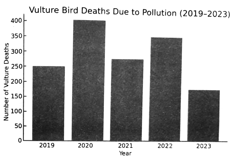
You can see that mortality peaked in 2020 and declined to its lowest in 2023.
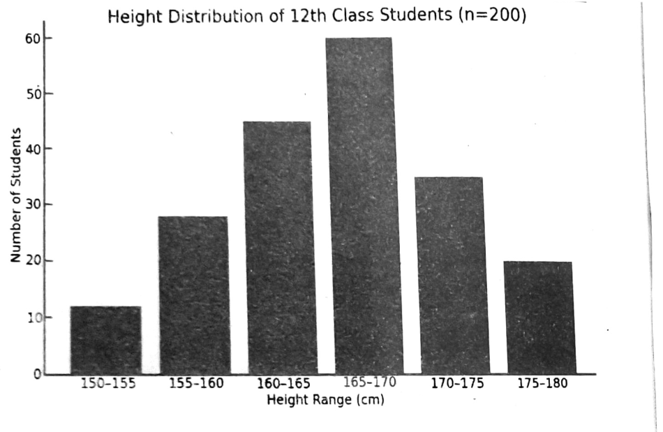
Height distribution in 200 students:
| Height Range (cm) | Number of Students |
|---|---|
| 150–155 | 12 |
| 155–160 | 28 |
| 160–165 | 45 |
| 165–170 | 60 |
| 170–175 | 35 |
| 175–180 | 20 |
| Total | 200 |